As global demand for seafood continues to rise, aquaculture—the farming of aquatic organisms—has emerged as a critical solution to meet nutritional needs while reducing pressure on wild fish stocks. But not all ocean waters are created equal. Marine species have specific environmental requirements, and identifying optimal farming locations requires careful spatial analysis of oceanographic conditions.
This analysis addresses a key question: Which U.S. West Coast Exclusive Economic Zone (EEZ) offers the most suitable habitat for commercially important shellfish species?
By combining sea surface temperature data, ocean depth measurements, and exclusive economic zone boundaries (EEZ), we can pinpoint the regions where aquaculture operations would have the greatest chance of success.
Why This Matters
Aquaculture is the fastest-growing food production sector globally, now accounting for over half of all fish consumed worldwide (FAO, 2022). Along the U.S. West Coast, shellfish farming represents a sustainable industry that provides economic benefits to coastal communities while offering ecosystem services like water filtration and habitat creation.
However, the success of aquaculture operations depends heavily on site selection. Species like oysters and abalone have narrow tolerance ranges for temperature and depth. Farming outside these optimal conditions leads to increased mortality, slower growth rates, and economic losses. Climate change further complicates this picture, as shifting ocean temperatures may alter which regions remain viable for specific species (Froehlich et al., 2018).
Understanding current habitat suitability is therefore essential for:
Industry planning: Guiding investment decisions for aquaculture operations
Regulatory management: Informing marine spatial planning within EEZs
Climate adaptation: Establishing baselines to track future habitat shifts
Data Sources
This analysis integrates three primary datasets:
Dataset
Source
Description
Sea Surface Temperature
NOAA
Average annual SST rasters (2008-2012)
Bathymetry
General Bathymetric Chart of the Oceans (GEBCO)
Ocean depth measurements
Exclusive Economic Zones
Marine Regions
West Coast EEZ boundary polygons
Species-specific temperature and depth requirements were obtained from SeaLifeBase, a global database of marine life information.
The Approach: Habitat Suitability Modeling
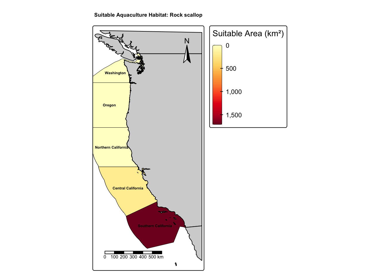
The analysis follows a systematic workflow that identifies suitable aquaculture locations. Let’s break it down step by step using the Rock scallop (Crassedoma giganteum) as an example. The Rock scallop prefers temperate water temperatures of about 13–22°C and shallower waters down to 45 meters.
Define species requirements: Set suitable sea surface temperature (°C) and depth ranges (m). Then identify the input layers (SST rasters, depth rasters, EEZ polygons). This anchors all further processing to the species’ physiological needs.
Reclassify environmental layers: Use reclassification matrices to convert continuous SST and depth into binary masks: values inside the acceptable range get a 1 (suitable) and everything else a 0 (unsuitable). For SST, the matrix maps anything below sst_min or above sst_max to 0, and values between to 1; for depth, the matrix does the same with depth_min and depth_max. Calling classify() with these matrices produces yes/no suitability rasters.
Overlay analysis: Combine the SST and depth masks to keep only cells that satisfy both criteria. The product of the two binary layers identifies candidate habitat cells.
Zonal statistics: Quantify suitable area by EEZ. Align projections, mask suitability to EEZ boundaries, convert EEZ polygons to a raster of IDs, multiply suitability by cell area (km²), and sum within each zone. This produces a ranked table of suitable area per EEZ, turning raster cells of suitability into regional metrics that we can visualize.
Show code
eez_data <-st_transform(eez_data, crs(suitable_cells))suitable_masked <-mask(suitable_cells, vect(eez_data))eez_rast <-rasterize(vect(eez_data), suitable_masked[[1]], field ="rgn")cell_area <-cellSize(suitable_masked, unit ="km")suitable_area_rast <- suitable_masked * cell_areatotal_area_per_eez <-zonal(suitable_area_rast, eez_rast, fun ="sum", na.rm =TRUE)colnames(total_area_per_eez) <-c("Region", "Suitable Area (km2)")ranked_eez <- total_area_per_eez[order(-total_area_per_eez$"Suitable Area (km2)"), ]
Visualization: Join the computed suitable area back to the EEZ polygons and map the results. The map shades EEZs by suitable area (km²), adds basemap context, and labels regions for clear regional comparison of habitat suitability.
Suitability for Rock scallop aquaculture across West Coast EEZs. Southern California is the most suitable region for this species.
Key Finding: Due to the Rock scallops warmer temperature preference, Southern California is shown to have the most suitable area for Rock scallop aquaculture.
Creating a Function
That workflow works great for identifying suitable aquaculture locations for an individual species, but it takes a lot of code. By combining each step into a function, additional species can be analyzed in one line of code, determining their most suitable zone quickly to aid in site selection. Included here is the function code that replaces the first step with suitability parameters and a Roxygen skeleton to provide function documentation.
Show code
#' @title Mapping Potential Aquaculture for species in West Coast Exclusive Economic Zones#' @author Lucian Scher#' @param species_name Name of species (Scientific or Common)#' @param sst_min Minimum of temperature range (Degrees Celsius)#' @param sst_max Maximum of temperature range (Degrees Celsius)#' @param depth_min Minimum of depth range negative for underwater (Meters)#' @param depth_max Maximum of depth range 0 for sea-level (Meters)#' *Optional Parameters:* to update SST, depth or EEZ data in case of changes: #' Default is data used this repository. #' Will need to re-prepare and re-process if neccessary to change these.#' @param sst_data Sea Surface Temperature Data#' @param depth_data Bathymetry data#' @param eez_data Exclusive Economic Zones#'#' @returns Map of EEZ regions colored by amount of suitable area for given species #' (species name included in map title)#| label: suitability-function# 1. Define species requirementsmap_species_suitability <-function(species_name, sst_min, sst_max, depth_min, depth_max,sst_data = mean_sst,depth_data = depth_resampled,eez_data = eez) {# 2. Reclassify environmental layers sst_rcl <-matrix(c(-Inf, sst_min, 0, sst_min, sst_max, 1, sst_max, Inf, 0), ncol =3, byrow =TRUE) depth_rcl <-matrix(c(-Inf, depth_min, 0, depth_min, depth_max, 1, depth_max, Inf, 0), ncol =3, byrow =TRUE)# Reclassify to binary suitability sst_bin <-classify(sst_data, rcl = sst_rcl) depth_bin <-classify(depth_data, rcl = depth_rcl) depth_stack <-rep(depth_bin, nlyr(sst_bin))# 3. Overlay analysis# Identify suitable cells suitable_cells <-lapp(c(sst_bin, depth_stack), fun =function(sst, depth) sst * depth)# 4. Zonal statistics# Match CRS eez_data <-st_transform(eez_data, crs(suitable_cells))# Mask to EEZ and rasterize suitable_masked <-mask(suitable_cells, vect(eez_data)) eez_rast <-rasterize(vect(eez_data), suitable_masked[[1]], field ="rgn")# Calculate suitable area per EEZ cell_area <-cellSize(suitable_masked, unit ="km") suitable_area_rast <- suitable_masked * cell_area total_area_per_eez <-zonal(suitable_area_rast, eez_rast, fun ="sum", na.rm =TRUE)# Change Column names for mappingcolnames(total_area_per_eez) <-c("Region", "Suitable Area (km2)")# Order largest to smallest ranked_eez <- total_area_per_eez[order(-total_area_per_eez$"Suitable Area (km2)"), ]# Round up decimals ranked_eez$"Suitable Area (km2)"<-round(ranked_eez$"Suitable Area (km2)", 1)# 5. Visualization# Add suitable area to EEZ polygons eez_data$"Suitable Area (km2)"<-setNames(ranked_eez$"Suitable Area (km2)", ranked_eez$Region)[eez_data$rgn]# Get land polygons cropped to EEZ extent with buffer land <-ne_countries(scale ="medium", returnclass ="sf") eez_bbox <-st_bbox(eez_data) eez_bbox[c("xmin", "ymin")] <- eez_bbox[c("xmin", "ymin")] -2 eez_bbox[c("xmax", "ymax")] <- eez_bbox[c("xmax", "ymax")] +2 land_cropped <-st_crop(land, eez_bbox)# Create and display map map <-tm_shape(land_cropped) +tm_polygons(fill ="lightgray", col ="black", lwd =1) +tm_shape(eez_data) +tm_polygons(fill ="Suitable Area (km2)", fill.scale =tm_scale_continuous(values ="brewer.yl_or_rd"),fill.legend =tm_legend(title ="Suitable Area (km²)"),col ="black", lwd =0.5) +tm_text("rgn", size =0.4, col ="black", fontface ="bold", remove.overlap =TRUE, auto.placement =TRUE) +tm_title(text =paste("Suitable Aquaculture Habitat:", species_name), size =0.7, fontface ="bold") +tm_scalebar(position =c("left", "bottom")) +tm_compass(position =c("right", "top")) +tm_layout(legend.outside =TRUE, legend.outside.position ="right")print(map)return(invisible(map))}
Results
Function testing on three different species.
Case Study 1: Oysters (General)
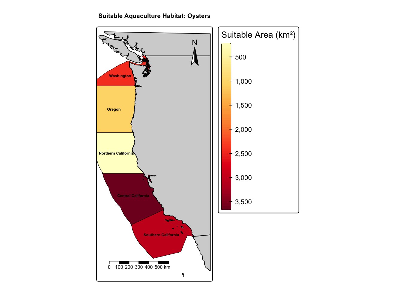
Oysters (Crassostrea spp.) are among the most economically important aquaculture species on the West Coast. They thrive in waters with temperatures between 11–30°C and depths from the surface down to 70 meters.
Figure 1: Habitat suitability for oyster aquaculture across West Coast EEZs. Central California emerges as the region with the greatest suitable area.
Key Finding: Central California offers the most extensive suitable habitat for general oyster farming, with its combination of moderate temperatures and extensive shallow coastal waters.
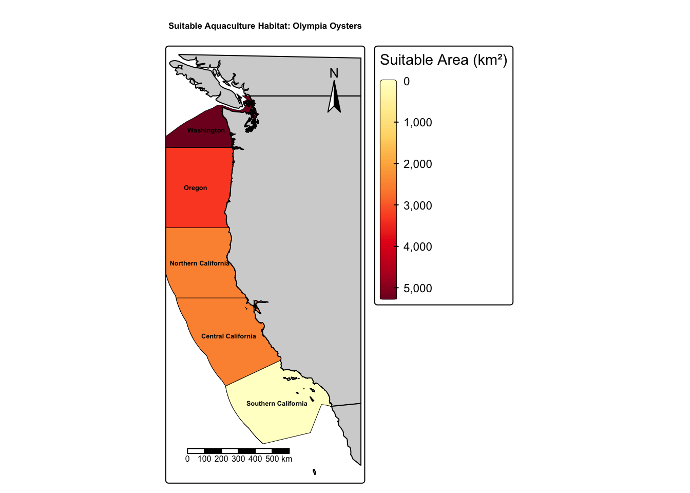
Case Study 2: Olympia Oysters (Ostrea lurida)
The Olympia oyster is the only oyster species native to the West Coast and has significant ecological and cultural value. However, it has much narrower temperature requirements (10–12°C) compared to other oyster species but similar depths (down to 71 meters).
Figure 2: Habitat suitability for Olympia oyster aquaculture. Washington’s cooler waters provide the most suitable conditions for this native species.
Key Finding: Washington emerges as the optimal region for Olympia oyster restoration and aquaculture efforts, reflecting the species’ preference for cooler northern waters.
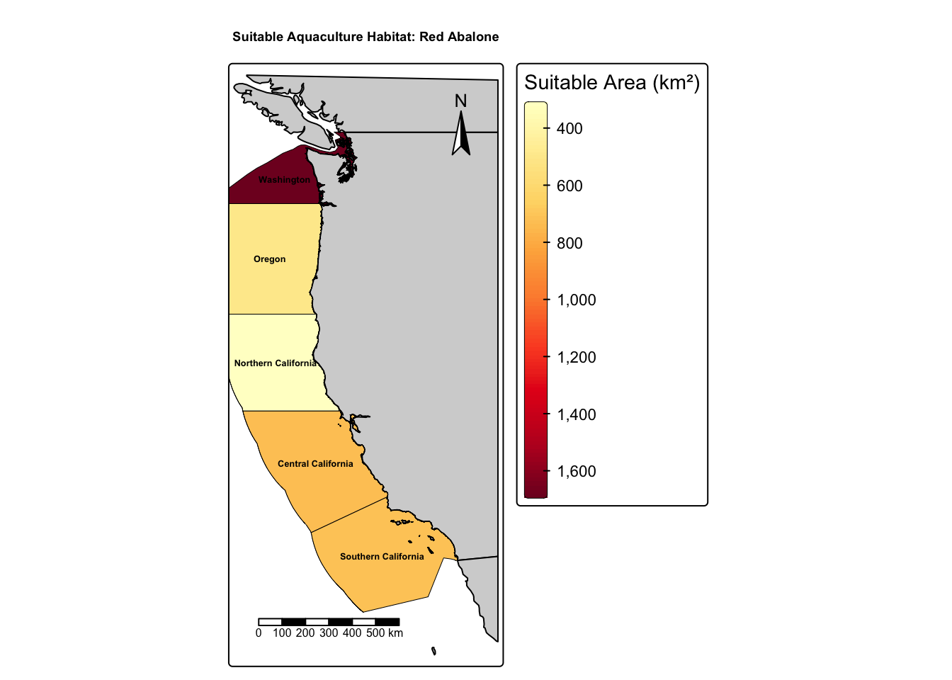
Case Study 3: Red Abalone (Haliotis rufescens)
Red abalone are prized for their meat and shells but have experienced dramatic population declines due to overharvesting and disease. They prefer temperatures between 8–18°C and shallower depths (down to 24 meters).
Figure 3: Habitat suitability for red abalone aquaculture. Washington provides the largest area of suitable habitat based on temperature and depth requirements.
Key Finding: Washington’s cooler waters and suitable bathymetry make it the most promising region for red abalone aquaculture development.
Conclusions
This analysis reveals distinct spatial patterns in aquaculture suitability across the West Coast:
Species
Optimal EEZ
Temperature Range
Depth Range
Oysters (general)
Central California
11–30°C
0–70m
Olympia Oyster
Washington
10–12°C
0–71m
Red Abalone
Washington
8–18°C
0–24m
Washington’s cooler waters make it particularly valuable for temperature-sensitive species, while Central California’s warmer and more extensive shallow areas favor species with broader thermal tolerance.
Limitations & Future Directions
This analysis provides a useful first approximation, but several factors warrant consideration:
Temporal variability: SST data represents a 5-year average (2008–2012); seasonal and interannual variability could affect site-specific suitability
Additional parameters: Factors like salinity, chlorophyll concentration, current patterns, and substrate type also influence aquaculture success
Climate projections: Future analyses should incorporate climate model projections to assess long-term viability
Regulatory constraints: Not all suitable areas may be available for aquaculture due to existing uses or protected status
Despite these limitations, spatial habitat suitability modeling provides an essential foundation for sustainable aquaculture development along the West Coast.
References
FAO. (2022). The State of World Fisheries and Aquaculture 2022: Towards Blue Transformation. Food and Agriculture Organization of the United Nations. https://www.fao.org/publications/sofia/2022/en/
Froehlich, H. E., Gentry, R. R., & Halpern, B. S. (2018). Global change in marine aquaculture production potential under climate change. Nature Ecology & Evolution, 2(11), 1745–1750. https://doi.org/10.1038/s41559-018-0669-1
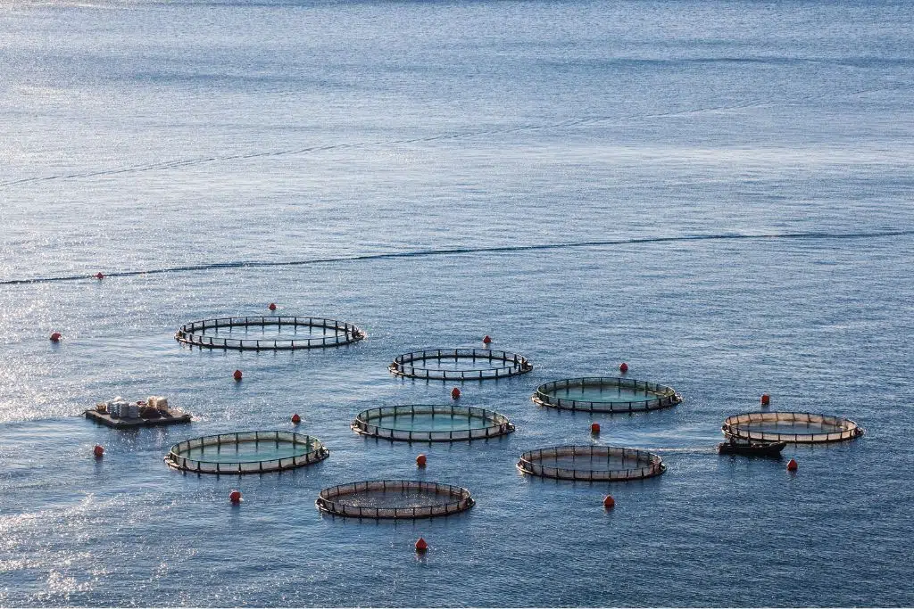 Image Credits: