library(tidyverse)
library(here)
library(readxl)
library(scales)
library(sf)
library(ggnewscale)
library(ggrepel)
library(treemapify)
library(haven)
library(lubridate)
library(patchwork)
knitr::opts_chunk$set(dpi = 150)
# --- 1. Setup & Color Palette ---
okabe_ito_11 <- c("#F0E442", "#009E73", "#E69F00", "#CC79A7", "#0072B2",
"#117733", "#D55E00", "#004E89", "#56B4E9", "#442288", "#999999")
make_top10_basin_palette <- function(top10_basin_names) {
if (length(top10_basin_names) != 10) {
stop("make_top10_basin_palette() expects exactly 10 basin names.")
}
setNames(okabe_ito_11, c(paste0(1:10, ". ", top10_basin_names), "Other basins"))
}
# --- 2. Data Wrangling (FHReD & Basins) ---
xl_path <- here("posts/hydro_infographic/data/FHReD_2015_future_dams_Zarfl_et_al_beta_version/FHReD_2015_future_dams_Zarfl_et_al_beta_version.xlsx")
future <- read_xlsx(xl_path, sheet = 2)
future_geo <- future %>%
filter(!is.na(`Capacity (MW)`), !is.na(LAT_cleaned), !is.na(Lon_Cleaned)) %>%
mutate(
basin = coalesce(`Major Basin`, "Other basins"),
basin = stringr::str_replace_all(basin, "Ganges - Bramaputra", "Ganges - Brahmaputra")
)
basin_mw <- future_geo %>%
group_by(basin) %>%
summarise(basin_mw_total = sum(`Capacity (MW)`, na.rm = TRUE), .groups = "drop") %>%
arrange(desc(basin_mw_total)) %>%
mutate(rank = row_number())
top_basins <- basin_mw %>% slice_head(n = 10) %>% pull(basin)
basin_palette <- make_top10_basin_palette(top_basins)
future_geo <- future_geo %>%
left_join(basin_mw, by = "basin") %>%
mutate(
basin_ranked = if_else(
basin %in% top_basins,
paste0(match(basin, top_basins), ". ", basin),
"Other basins"
),
basin_ranked = factor(basin_ranked, levels = names(basin_palette))
)
# --- 3. World Map Visualization ---
biome_ci <- tribble(
~biome, ~ci_median,
"Tundra", 43.8,
"Boreal", 104.4,
"Temperate", 54.8,
"Tropical", 91.0
)
assign_biome <- function(lat) {
case_when(
lat >= 60 | lat <= -60 ~ "Tundra",
(lat >= 50 & lat < 60) | (lat <= -50 & lat > -60) ~ "Boreal",
(lat >= 23 & lat < 50) | (lat <= -23 & lat > -50) ~ "Temperate",
lat > -23 & lat < 23 ~ "Tropical",
TRUE ~ NA_character_
)
}
future_geo_map <- future_geo %>%
mutate(biome = assign_biome(LAT_cleaned)) %>%
left_join(biome_ci, by = "biome")
lat_bands <- tribble(
~ymin, ~ymax, ~biome,
-90, -60, "Tundra",
-60, -50, "Boreal",
-50, -23, "Temperate",
-23, 23, "Tropical",
23, 50, "Temperate",
50, 60, "Boreal",
60, 90, "Tundra"
) %>%
left_join(biome_ci, by = "biome")
pal_ci <- c("Tundra" = "#D8E9D9", "Boreal" = "#E0E0E0", "Temperate" = "#A8D1AA", "Tropical" = "#58A86F")
basins_lev02 <- readRDS(here("posts/hydro_infographic/data/basins_lev02_geom.rds")) %>%
sf::st_as_sf()
if (is.na(sf::st_crs(basins_lev02))) sf::st_crs(basins_lev02) <- 4326
sf::sf_use_s2(FALSE)
basins_lev02 <- sf::st_make_valid(basins_lev02) %>%
sf::st_collection_extract("POLYGON") %>%
sf::st_cast("MULTIPOLYGON", warn = FALSE)
future_pts <- future_geo_map %>%
st_as_sf(coords = c("Lon_Cleaned", "LAT_cleaned"), crs = 4326, remove = FALSE)
future_with_basin <- st_join(future_pts, basins_lev02 %>% select(hybas_id), left = FALSE)
sf::sf_use_s2(TRUE)
basin_stats <- future_with_basin %>%
st_drop_geometry() %>%
group_by(hybas_id) %>%
summarise(future_mw = sum(`Capacity (MW)`, na.rm = TRUE), .groups = "drop")
basin_map <- basins_lev02 %>%
left_join(basin_stats, by = "hybas_id") %>%
mutate(future_mw = replace_na(future_mw, 0))
basin_labels <- future_geo_map %>%
filter(basin %in% top_basins) %>%
group_by(basin) %>%
summarise(anchor_x = median(Lon_Cleaned, na.rm = TRUE), anchor_y = median(LAT_cleaned, na.rm = TRUE), .groups = "drop") %>%
left_join(basin_mw %>% filter(rank <= 10) %>% transmute(basin, label_rank = paste0(rank, ". ", basin)), by = "basin") %>%
mutate(
label = label_rank,
nudge_x = case_when(basin == "Yangtze" ~ 60, basin == "Mekong" ~ 40, basin == "Amazon" ~ 30, basin == "La Plata" ~ 25, basin == "Congo" ~ -30, basin == "Nile" ~ 20, basin == "Irrawaddy" ~ -15, basin == "Salween" ~ 40, basin == "Indus" ~ -10, basin == "Ganges - Brahmaputra" ~ 10, TRUE ~ 0),
nudge_y = case_when(basin == "Yangtze" ~ 10, basin == "Mekong" ~ -15, basin == "Amazon" ~ 10, basin == "La Plata" ~ -5, basin == "Congo" ~ -15, basin == "Nile" ~ -5, basin == "Irrawaddy" ~ -25, basin == "Salween" ~ -5, basin == "Indus" ~ 10, basin == "Ganges - Brahmaputra" ~ 25, TRUE ~ 0)
)
p_map <- ggplot() +
geom_rect(data = lat_bands, aes(xmin = -180, xmax = 180, ymin = ymin, ymax = ymax, fill = biome), color = NA, alpha = 0.35) +
scale_fill_manual(values = pal_ci, name = "Biome") +
ggnewscale::new_scale_fill() +
geom_sf(data = basin_map, aes(fill = future_mw), color = NA, inherit.aes = FALSE) +
scale_fill_gradient(low = "grey95", high = "grey20", trans = "sqrt", labels = comma, name = "Basin capacity (MW)") +
geom_point(data = future_geo_map, aes(x = Lon_Cleaned, y = LAT_cleaned, size = `Capacity (MW)`, color = basin_ranked), shape = 16, alpha = 0.85, inherit.aes = FALSE) +
scale_size_continuous(range = c(1.2, 9), labels = comma, name = "Dam capacity (MW)") +
scale_color_manual(values = basin_palette, guide = "none") +
ggrepel::geom_text_repel(data = basin_labels, aes(x = anchor_x, y = anchor_y, label = label), color = "#000000", size = 3, fontface = "bold", family = "Times New Roman", lineheight = 0.9, seed = 123, nudge_x = basin_labels$nudge_x, nudge_y = basin_labels$nudge_y, box.padding = 0.5, point.padding = 0.5, segment.color = "#000000", segment.size = 0.4, segment.alpha = 0.95, min.segment.length = 0, inherit.aes = FALSE) +
coord_sf(xlim = c(-180, 180), ylim = c(-60, 75)) +
theme_minimal(base_size = 9) +
theme(panel.grid = element_blank(), axis.text = element_blank(), axis.ticks = element_blank(), legend.text = element_text(family = "Times New Roman"), legend.title = element_text(face = "bold", family = "Times New Roman"))
# --- 4. Treemap Visualization ---
treemap_data <- future_geo %>%
group_by(basin_ranked) %>%
summarise(mw = sum(`Capacity (MW)`, na.rm = TRUE), .groups = "drop") %>%
filter(mw > 0) %>%
mutate(basin_name = as.character(basin_ranked), mw_label = paste0("(", scales::comma(round(mw)), " MW)"))
p_treemap <- ggplot(treemap_data, aes(area = mw, fill = basin_ranked)) +
geom_treemap(layout = "squarified", color = "white", linewidth = 0.5) +
geom_treemap_text(aes(label = basin_name), place = "centre", grow = TRUE, family = "Times New Roman", color = "black", min.size = 1, padding.y = grid::unit(2, "mm")) +
geom_treemap_text(aes(label = mw_label), place = "bottom", size = 10, family = "Times New Roman", fontface = "plain", color = "black", min.size = 1, padding.y = grid::unit(2, "mm")) +
scale_fill_manual(values = basin_palette, guide = "none") +
theme_minimal() + theme(legend.position = "none")
# --- 5. Hydropower Sun (Timing) ---
dta <- read_dta(here::here("posts/hydro_infographic/data/marginal-generation-offsets-data.dta"))
inner_radius <- 1.5
inner_month <- dta %>%
mutate(month_num = month(dt), month_lab = factor(month.abb[month_num], levels = month.abb)) %>%
group_by(month_lab) %>%
summarise(h_mean = mean(h, na.rm = TRUE), .groups = "drop") %>%
mutate(h_norm = h_mean / max(h_mean, na.rm = TRUE)) %>%
inner_join(tibble(month_lab = factor(month.abb, levels = month.abb), x_center = seq(1, 23, by = 2)), by = "month_lab")
outer_hour <- dta %>%
mutate(hour = hour(dt)) %>%
group_by(hour) %>%
summarise(h_mean = mean(h, na.rm = TRUE), .groups = "drop") %>%
mutate(h_norm = h_mean / max(h_mean, na.rm = TRUE), hour_rot = (hour - 12) %% 24, inner_r = inner_radius + 0.1, outer_r = inner_r + 0.9 * h_norm)
p_sun <- ggplot() +
geom_col(data = inner_month, aes(x = x_center, y = inner_radius, fill = h_norm), width = 2, color = NA) +
geom_segment(data = outer_hour, aes(x = hour_rot, xend = hour_rot, y = inner_r, yend = outer_r, color = h_norm), linewidth = 1.0) +
coord_polar(theta = "x", start = 0) +
scale_colour_gradientn(colours = c("#fff7bc", "#993404"), name = "Avg hydro") +
scale_fill_gradientn(colours = c("#fff7bc", "#993404"), guide = "none") +
theme_minimal() + theme(axis.text = element_blank(), panel.grid = element_blank())
# --- 6. Capacity vs Carbon Threshold ---
nze <- read_csv(here("posts/hydro_infographic/data/NZE2021_AnnexA.csv"), show_col_types = FALSE)
shares <- read_csv(here("posts/hydro_infographic/data/share_failing_80kg.csv"), show_col_types = FALSE)
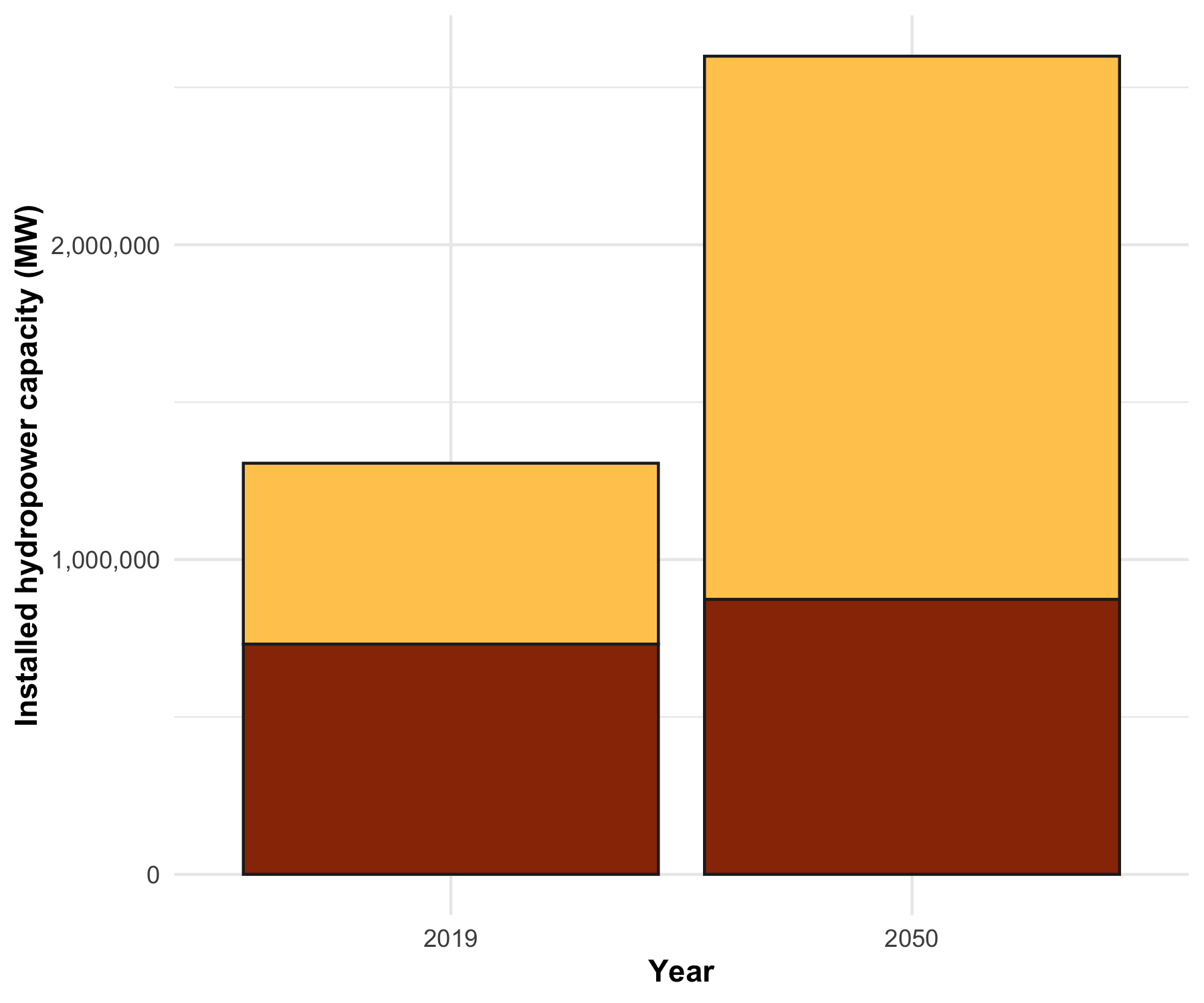
capacity_split <- nze %>%
filter(Product == "Hydro", Flow == "Installed total power capacity", Unit == "GW", Year %in% c(2019, 2050)) %>%
mutate(Hydro_MW = Value * 1000, group = if_else(Year == 2019, "Existing dams", "Future dams")) %>%
left_join(shares, by = "group") %>%
mutate(MW_above = Hydro_MW * (pct_above_80 / 100), MW_below = Hydro_MW * (pct_below_80 / 100)) %>%
pivot_longer(cols = c(MW_above, MW_below), names_to = "segment", values_to = "MW") %>%
mutate(segment = if_else(segment == "MW_above", "Above 80 kg CO2e/MWh", "Below 80 kg CO2e/MWh"), Year = factor(Year))
p_capacity_threshold <- ggplot(capacity_split, aes(x = Year, y = MW, fill = segment)) +
geom_col(color = "#222222") +
scale_fill_manual(values = c("Below 80 kg CO2e/MWh" = "#993404", "Above 80 kg CO2e/MWh" = "#FFCA5C")) +
theme_minimal()